
Practice Free Databricks Certified Professional Data Engineer Exam Online Questions
Each configuration below is identical to the extent that each cluster has 400 GB total of RAM, 160 total cores and only one Executor per VM.
Given a job with at least one wide transformation, which of the following cluster configurations will result in maximum performance?
- A . • Total VMs: 1• 400 GB per Executor• 160 Cores / Executor
- B . • Total VMs: 8• 50 GB per Executor• 20 Cores / Executor
- C . • Total VMs: 4• 100 GB per Executor• 40 Cores/Executor
- D . • Total VMs: 2• 200 GB per Executor• 80 Cores / Executor
B
Explanation:
This is the correct answer because it is the cluster configuration that will result in maximum performance for a job with at least one wide transformation. A wide transformation is a type of transformation that requires shuffling data across partitions, such as join, groupBy, or orderBy. Shuffling can be expensive and time-consuming, especially if there are too many or too few partitions. Therefore, it is important to choose a cluster configuration that can balance the trade-off between parallelism and network overhead. In this case, having 8 VMs with 50 GB per executor and 20 cores per executor will create 8 partitions, each with enough memory and CPU resources to handle the shuffling efficiently. Having fewer VMs with more memory and cores per executor will create fewer partitions, which will reduce parallelism and increase the size of each shuffle block. Having more VMs with less memory and cores per executor will create more partitions, which will increase parallelism but also increase the network overhead and the number of shuffle files.
Verified Reference: [Databricks Certified Data Engineer Professional], under “Performance Tuning” section; Databricks Documentation, under “Cluster configurations” section.
Although the Databricks Utilities Secrets module provides tools to store sensitive credentials and avoid accidentally displaying them in plain text users should still be careful with which credentials are stored here and which users have access to using these secrets.
Which statement describes a limitation of Databricks Secrets?
- A . Because the SHA256 hash is used to obfuscate stored secrets, reversing this hash will display the value in plain text.
- B . Account administrators can see all secrets in plain text by logging on to the Databricks Accounts console.
- C . Secrets are stored in an administrators-only table within the Hive Metastore; database administrators have permission to query this table by default.
- D . Iterating through a stored secret and printing each character will display secret contents in plain text.
- E . The Databricks REST API can be used to list secrets in plain text if the personal access token has proper credentials.
E
Explanation:
This is the correct answer because it describes a limitation of Databricks Secrets. Databricks Secrets is a module that provides tools to store sensitive credentials and avoid accidentally displaying them in plain text. Databricks Secrets allows creating secret scopes, which are collections of secrets that can be accessed by users or groups. Databricks Secrets also allows creating and managing secrets using
the Databricks CLI or the Databricks REST API. However, a limitation of Databricks Secrets is that the Databricks REST API can be used to list secrets in plain text if the personal access token has proper credentials. Therefore, users should still be careful with which credentials are stored in Databricks Secrets and which users have access to using these secrets.
Verified Reference: [Databricks Certified Data Engineer Professional], under “Databricks Workspace” section; Databricks Documentation, under “List secrets” section.
A data engineer is creating a data ingestion pipeline to understand where customers are taking their rented bicycles during use. The engineer noticed that, over time, data being transmitted from the bicycle sensors fail to include key details like latitude and longitude. Downstream analysts need both the clean records and the quarantined records available for separate processing.
The data engineer already has this code:
import dlt
from pyspark.sql.functions import expr
rules = {
"valid_lat": "(lat IS NOT NULL)",
"valid_long": "(long IS NOT NULL)"
}
quarantine_rules = "NOT({})".format(" AND ".join(rules.values()))
@dlt.view
def raw_trips_data():
return spark.readStream.table("ride_and_go.telemetry.trips")
How should the data engineer meet the requirements to capture good and bad data?
- A . @dlt.table(name="trips_data_quarantine")def trips_data_quarantine():return (spark.readStream.table("raw_trips_data").filter(expr(quarantine_rules)))
- B . @[email protected]_or_drop("lat_long_present", "(lat IS NOT NULL AND long IS NOT NULL)")def trips_data_quarantine():return spark.readStream.table("ride_and_go.telemetry.trips")
- C . @[email protected]_all_or_drop(rules)def trips_data_quarantine():return
spark.readStream.table("raw_trips_data") - D . @dlt.table(partition_cols=["is_quarantined", ])@dlt.expect_all(rules)def trips_data_quarantine():return (spark.readStream.table("raw_trips_data").withColumn("is_quarantined", expr(quarantine_rules)))
A
Explanation:
The requirement is that both valid (good) and invalid (bad) records must be captured and available separately for downstream processing. Invalid records should not simply be dropped; they must be quarantined in a dedicated table.
In Databricks Lakeflow Declarative Pipelines (DLT), this is achieved by creating separate output tables:
One table for valid records (Silver table) that pass the expectations.
Another quarantine table that explicitly captures records failing the expectations.
Option A correctly implements this by:
Declaring a DLT table trips_data_quarantine.
Using .filter(expr(quarantine_rules)) to isolate invalid records (records where latitude or longitude is NULL).
This ensures analysts can query both good records (from the main Silver pipeline table) and bad records (from the quarantine table).
Why not the others?
B: Uses @dlt.expect_or_drop, which drops invalid records instead of quarantining them. This violates the requirement that quarantined data should be available.
C: Same as B, but applies expectations in bulk with expect_all_or_drop. Again, bad data is dropped, not quarantined.
D: Adds an is_quarantined flag in the same table. While it marks bad records, it does not separate them into a distinct quarantine table as required by the business use case.
Therefore, Option A is the only solution aligned with Databricks documentation for quarantining invalid data into a dedicated table while keeping valid data in the main pipeline.
A data engineer is configuring a Databricks Asset Bundle to deploy a job with granular permissions.
The requirements are:
Grant the data-engineers group CAN_MANAGE access to the job.
Ensure the auditors group can view the job but not modify or run it.
Avoid granting unintended permissions to other users or groups.
How should the data engineer deploy the job while meeting the requirements?
- A . resources:
jobs:
my-job:
name: data-pipeline
tasks: (…)
job_clusters: (…)
permissions:
– group_name: data-engineers level: CAN_MANAGE
– group_name: auditors
level: CAN_VIEW - B . resources:
jobs:
my-job:
name: data-pipeline
tasks: (…)
job_clusters: (…)
permissions:
– group_name: data-engineers level: CAN_MANAGE
– group_name: auditors
level: CAN_VIEW - C . resources:
jobs:
my-job:
name: data-pipeline
tasks: […]
job_clusters: […]
permissions:
– group_name: data-engineers level: CAN_MANAGE permissions:
– group_name: auditors
level: CAN_VIEW - D . permissions:
– group_name: data-engineers level: CAN_MANAGE
– group_name: auditors
level: CAN_VIEW
resources:
jobs:
my-job:
name: data-pipeline
tasks: […]
job_clusters: […]
B
Explanation:
Databricks documents that resource-specific permissions for bundle resources can be defined under the resource itself, such as resources.jobs.<job>.permissions, using group_name and level. The documented syntax supports CAN_VIEW, CAN_MANAGE, and related permission levels, which matches option
B. (Databricks Documentation)
Option C is invalid because it repeats the permissions key incorrectly.
Option D applies top-level permissions more broadly across bundle resources instead of scoping them specifically to the job, which does not best satisfy the “avoid unintended permissions” requirement.
Option B is therefore the correct and properly scoped configuration. (Databricks Documentation)
A junior data engineer is working to implement logic for a Lakehouse table named silver_device_recordings. The source data contains 100 unique fields in a highly nested JSON structure.
The silver_device_recordings table will be used downstream for highly selective joins on a number of fields, and will also be leveraged by the machine learning team to filter on a handful of relevant fields, in total, 15 fields have been identified that will often be used for filter and join logic.
The data engineer is trying to determine the best approach for dealing with these nested fields before declaring the table schema.
Which of the following accurately presents information about Delta Lake and Databricks that may Impact their decision-making process?
- A . Because Delta Lake uses Parquet for data storage, Dremel encoding information for nesting can be directly referenced by the Delta transaction log.
- B . Tungsten encoding used by Databricks is optimized for storing string data: newly-added native support for querying JSON strings means that string types are always most efficient.
- C . Schema inference and evolution on Databricks ensure that inferred types will always accurately match the data types used by downstream systems.
- D . By default Delta Lake collects statistics on the first 32 columns in a table; these statistics are leveraged for data skipping when executing selective queries.
D
Explanation:
Delta Lake, built on top of Parquet, enhances query performance through data skipping, which is based on the statistics collected for each file in a table. For tables with a large number of columns, Delta Lake by default collects and stores statistics only for the first 32 columns. These statistics include min/max values and null counts, which are used to optimize query execution by skipping irrelevant data files. When dealing with highly nested JSON structures, understanding this behavior is crucial for schema design, especially when determining which fields should be flattened or prioritized in the table structure to leverage data skipping efficiently for performance optimization.
: Databricks documentation on Delta Lake optimization techniques, including data skipping and statistics collection (https://docs.databricks.com/delta/optimizations/index.html).
A junior data engineer has been asked to develop a streaming data pipeline with a grouped aggregation using DataFrame df. The pipeline needs to calculate the average humidity and average temperature for each non-overlapping five-minute interval. Incremental state information should be maintained for 10 minutes for late-arriving data.
Streaming DataFrame df has the following schema:
"device_id INT, event_time TIMESTAMP, temp FLOAT, humidity FLOAT"
Code block:
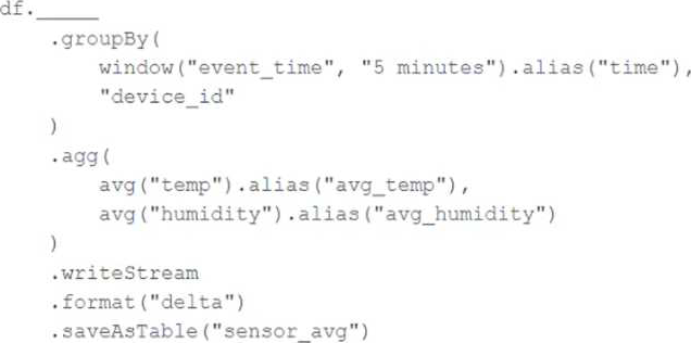
Choose the response that correctly fills in the blank within the code block to complete this task.
- A . withWatermark("event_time", "10 minutes")
- B . awaitArrival("event_time", "10 minutes")
- C . await("event_time + ‘10 minutes’")
- D . slidingWindow("event_time", "10 minutes")
- E . delayWrite("event_time", "10 minutes")
A
Explanation:
The correct answer is A. withWatermark(“event_time”, “10 minutes”). This is because the question asks for incremental state information to be maintained for 10 minutes for late-arriving data. The withWatermark method is used to define the watermark for late data. The watermark is a timestamp column and a threshold that tells the system how long to wait for late data. In this case, the watermark is set to 10 minutes. The other options are incorrect because they are not valid methods or syntax for watermarking in Structured Streaming.
Reference:
Watermarking: https://docs.databricks.com/spark/latest/structured-streaming/watermarks.html
Windowed aggregations: https://docs.databricks.com/spark/latest/structured-streaming/window-operations.html
A Structured Streaming job deployed to production has been experiencing delays during peak hours of the day. At present, during normal execution, each microbatch of data is processed in less than 3 seconds. During peak hours of the day, execution time for each microbatch becomes very inconsistent, sometimes exceeding 30 seconds. The streaming write is currently configured with a trigger interval of 10 seconds.
Holding all other variables constant and assuming records need to be processed in less than 10 seconds, which adjustment will meet the requirement?
- A . Decrease the trigger interval to 5 seconds; triggering batches more frequently allows idle executors to begin processing the next batch while longer running tasks from previous batches finish.
- B . Increase the trigger interval to 30 seconds; setting the trigger interval near the maximum execution time observed for each batch is always best practice to ensure no records are dropped.
- C . The trigger interval cannot be modified without modifying the checkpoint directory; to maintain the current stream state, increase the number of shuffle partitions to maximize parallelism.
- D . Use the trigger once option and configure a Databricks job to execute the query every 10 seconds; this ensures all backlogged records are processed with each batch.
- E . Decrease the trigger interval to 5 seconds; triggering batches more frequently may prevent records from backing up and large batches from causing spill.
D
Explanation:
The scenario presented involves inconsistent microbatch processing times in a Structured Streaming job during peak hours, with the need to ensure that records are processed within 10 seconds. The trigger once option is the most suitable adjustment to address these challenges:
Understanding Triggering Options:
Fixed Interval Triggering (Current Setup): The current trigger interval of 10 seconds may contribute to the inconsistency during peak times as it doesn’t adapt based on the processing time of the microbatches. If a batch takes longer to process, subsequent batches will start piling up, exacerbating the delays.
Trigger Once: This option allows the job to run a single microbatch for processing all available data and then stop. It is useful in scenarios where batch sizes are unpredictable and can vary significantly, which seems to be the case during peak hours in this scenario.
Implementation of Trigger Once:
Setup: Instead of continuously running, the job can be scheduled to run every 10 seconds using a Databricks job. This scheduling effectively acts as a custom trigger interval, ensuring that each execution cycle handles all available data up to that point without overlapping or queuing up additional executions.
Advantages: This approach allows for each batch to complete processing all available data before the next batch starts, ensuring consistency in handling data surges and preventing the system from being overwhelmed.
Rationale Against Other Options:
Option A and E (Decrease Interval): Decreasing the trigger interval to 5 seconds might exacerbate the problem by increasing the frequency of batch starts without ensuring the completion of previous batches, potentially leading to higher overhead and less efficient processing.
Option B (Increase Interval): Increasing the trigger interval to 30 seconds could lead to latency issues, as the data would be processed less frequently, which contradicts the requirement of processing records in less than 10 seconds.
Option C (Modify Partitions): While increasing parallelism through more shuffle partitions can improve performance, it does not address the fundamental issue of batch scheduling and could still lead to inconsistency during peak loads.
Conclusion:
By using the trigger once option and scheduling the job every 10 seconds, you ensure that each microbatch has sufficient time to process all available data thoroughly before the next cycle begins, aligning with the need to handle peak loads more predictably and efficiently.
Reference
Structured Streaming Programming Guide – Triggering
Databricks Jobs Scheduling
A data architect has heard about lake’s built-in versioning and time travel capabilities. For auditing purposes they have a requirement to maintain a full of all valid street addresses as they appear in the customers table.
The architect is interested in implementing a Type 1 table, overwriting existing records with new values and relying on Delta Lake time travel to support long-term auditing. A data engineer on the project feels that a Type 2 table will provide better performance and scalability.
Which piece of information is critical to this decision?
- A . Delta Lake time travel does not scale well in cost or latency to provide a long-term versioning solution.
- B . Delta Lake time travel cannot be used to query previous versions of these tables because Type 1 changes modify data files in place.
- C . Shallow clones can be combined with Type 1 tables to accelerate historic queries for long-term versioning.
- D . Data corruption can occur if a query fails in a partially completed state because Type 2 tables requires Setting multiple fields in a single update.
A
Explanation:
Delta Lake’s time travel feature allows users to access previous versions of a table, providing a powerful tool for auditing and versioning. However, using time travel as a long-term versioning solution for auditing purposes can be less optimal in terms of cost and performance, especially as the volume of data and the number of versions grow. For maintaining a full history of valid street addresses as they appear in a customers table, using a Type 2 table (where each update creates a new record with versioning) might provide better scalability and performance by avoiding the overhead associated with accessing older versions of a large table. While Type 1 tables, where existing records are overwritten with new values, seem simpler and can leverage time travel for auditing, the critical piece of information is that time travel might not scale well in cost or latency for long-term versioning needs, making a Type 2 approach more viable for performance and scalability.
Databricks Documentation on Delta Lake’s Time Travel: Delta Lake Time Travel
Databricks Blog on Managing Slowly Changing Dimensions in Delta Lake: Managing SCDs in Delta Lake
Which distribution does Databricks support for installing custom Python code packages?
- A . sbt
- B . CRAN
- C . CRAM
- D . nom
- E . Wheels
- F . jars
A data engineering team is configuring access controls in Databricks Unity Catalog. They grant the SELECT privilege on the sales catalog to the analyst_group, expecting that members of this group will automatically have SELECT access to all current and future schemas, tables, and views within the catalog.
What describes the privilege inheritance behavior in Unity Catalog?
- A . Granting SELECT at the catalog level applies to existing schemas and tables but not to those created in the future.
- B . Privileges in Unity Catalog do not cascade; SELECT must be explicitly granted on each schema and table, even if granted at the catalog level.
- C . Privileges granted at the schema level override any catalog-level privileges and prevent access unless explicitly revoked.
- D . Granting SELECT on a catalog automatically applies SELECT to all current and future schemas, tables, and views within that catalog.
B
Explanation:
In Unity Catalog, privileges are non-cascading―meaning that granting a privilege (like SELECT) on a catalog does not automatically grant the same privilege on contained objects (schemas, tables, or views). Each object type has its own independent access control hierarchy.
According to the Databricks access control documentation: “Privileges do not automatically cascade from catalog to schema or table levels.” Administrators must explicitly grant privileges on each level if users need access across objects. This design ensures tighter governance and least-privilege enforcement. Therefore, option B correctly describes Unity Catalog’s privilege model, while A and D incorrectly imply automatic inheritance.